Binning is a general term for grouping a dataset of N values into less than N discrete groups. These groups/bins may be spatial, temporal, or otherwise attribute-based. In this post I’m only talking about spatial (long-lat) and 2-dimensional attribute-based (scatterplot) bins. Such binnings may be thought of as 2D histograms. This may make more or less sense after what lies beneath.
If you’re just after that sweet honey that is my code, bear down on my Github repository for this project — hexbin-js.
Rectangular binning
The simplest 2D bin is rectangular. Indeed, for most purposes rectangular bins suffice, and their computational simplicity is a significant advantage.
The above is a shot from a little example I produced on jsFiddle, while learning Mike Bostock’s fantastic D3 JavaScript library for HTML and SVG data-binding and visualization. The example demonstrates the need for and the technique of 2D rectangular binning and aggregation.
Binning can be good for both the users and the creators/developers of static or interactive thematic maps or other visualizations. For the user, showing every single point can lead to cognitive overload, and may even be inaccurate, as overlapping points lead to a misreading of density.
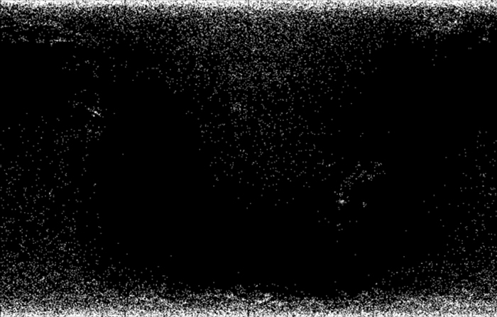
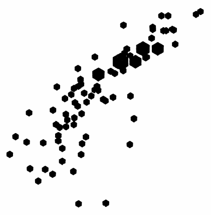
In the above image (from Antaeus Concepts) the data points are represented in black, and due to overlap the true concentration/density distribution is indiscernible from the graphic.
A binned representation may reveal patterns not readily seen in the raw point representation of the data (see Antaeus’ sunflower plot for the same data below). For the developer or cartographer, too, binning can present an advantage, chiefly in efficiency. Back in the day, manual cartographers probably weren’t too keen on drawing 10’s of 1000’s of data points — I’m guessing they’d rather do the cheap bin math so that they could then only draw 10’s or 100’s of uniformly-shaped bins to represent the same data.
Though we modern cartographers have fancy-fangled computers to draw our data points for us, even these beasts hiccup when asked to draw 10,000+ points at once. Hiccups are acceptable in static rendering, but not in real-time apps that employ animation (as even at just 5 frames per second, rendering 1000s of points each frame would prove intensive for even newer home desktops).
So anyway, binned representations can be beneficial for both users and creators. Below I’ll just describe one binning method (hexagon binning, or hexbinning), its implementation, and some examples.
Hexagonal binning
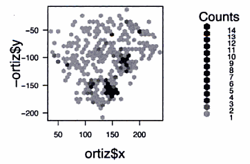
I first encountered hexagonal binning in the sweet 2006 O’Reilly book by Joseph Adler, Baseball Hacks. Adler demonstrates the need for binning by showing a “spraychart” of David Ortiz’s 2003 balls-in-play.
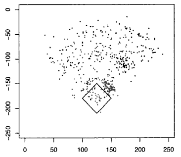
Adler writes,
Clearly, you can see that David Ortiz tends to hit balls more often to right field. Wouldn’t it be nice to have a cleaner way to see this density? We’ll use another visualization technique, called hexagonal binning, to get a clearer picture of where Ortiz’s hits land.
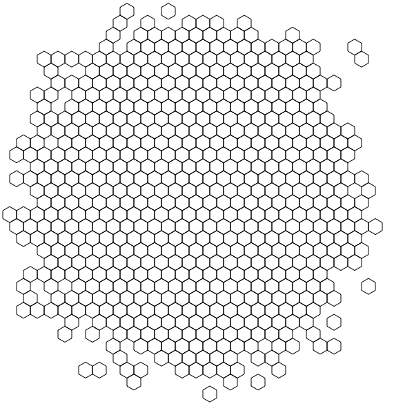
The idea of hexagonal binning is to break a two-dimensional plane into different bins. First, the bins make interlocking hexagons. It is possible to use squares (or interlocking triangles or another shape), but hexagons look “rounder” than squares.
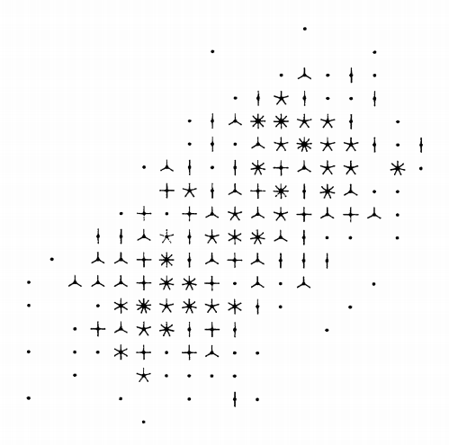
To turn his spraychart into hexbins, Adler used the hexbin package for R developed by Nicholas Lewin-Koh and Martin Maechler (inspired by Dan Carr’s work; more on this below).
Though unfortunately printed smaller in the book than the spraychart, I think the hexbin representation does effectively simplify the data while revealing patterns not easily retrieved from the full spraychart representation.
Hex history and theory
The technique of using interlocking hexagons to aggregate 2-dimensional data was first described in a 1987 paper by four Pacific Northwest Laboratory statisticians (D.B. Carr et al, “Scatterplot Matrix Techniques for Large N”). The authors note, though, that they were inspired by another binning technique — sunflower plots — described a few years earlier by William Cleveland and Robert McGill.
Cleveland and McGill (1984, “The Many Faces of a Scatterplot”) didn’t mention hexagons; indeed they specified that squares be used to bin the data, with each bin then being tranformed into a “sunflower”, with each “petal” representing a datum within the bin:
In their later 1987 paper, D.B. Carr et al suggested that hexagon-bin-based sunflowers represented the data more faithfully than the rectangular-bin version. They cite various reasons for this advantage, but I think it basically comes down to Joseph Adler’s later observation that “hexagons look rounder than squares”. Indeed, a regular tessellation of a 2D surface is not possible with polygons of greater than six sides, making the hexagonal tessellation the most efficient and compact division of 2D data space.
Besides hexbin sunflower plots, D.B. Carr et al note two other possible symbologies to employ once the data have been successfully hex-binned. To use thematic mapping parlance, the methods are proportional symbols and choropleth. These symbologies and other possibilities are discussed below.
Hexbin symbologies
Hexbinning consists of 1) laying a hexagonal grid or lattice atop a 2-dimensional field of data and 2) determining data point counts for each hexagon. This says nothing of the symbolization or representation method that can then be employed to communicate these counts to the graphic’s reader.
Sunflower plots
Sunflowers are likely the most complex symbology for representing hexbins, but I’m covering them first in this section because they actually inspired the hexbinning method itself.
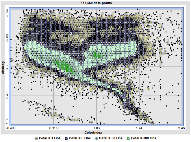
The above screenshot is from the Antaeus statistics project, and hexagonal sunflower plots have also been implemented within the popular Stata statistics package:
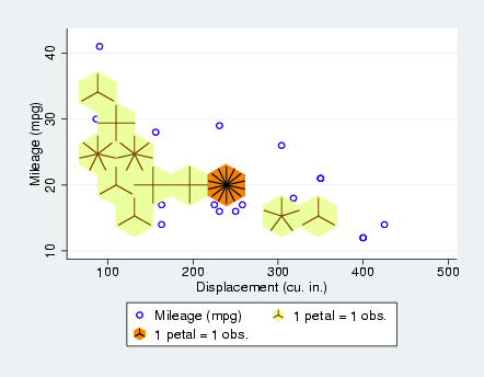
Whether square-bin or hexbin-based, these sunflower plots are notable for allowing the user to simultaneously view generalities and retrieve specifics. A higher number of “petals” leads to a darker hexagon, and clusters of such hexagons will reveal the overall trend of the data. At the same time, individual petals can be counted to determine the exact number of data lying within each hexagonal bin.
Proportional symbol
The choropleth and proportional symbologies don’t really need any explanation here, so images should suffice.
Choropleth
Multivariate
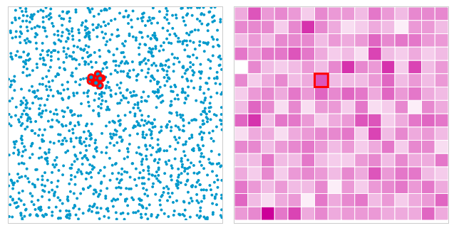
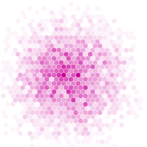
In a multivariate hexbin representation, the secondary variable can be anything, though the sum or average of some attribute of the binned points within each hex would be typical.
In the below, a bivariate symbology is shown, though in this case the variable distribution represented by color value/saturation is the same as that represented by size (making this a redundant symbolization).
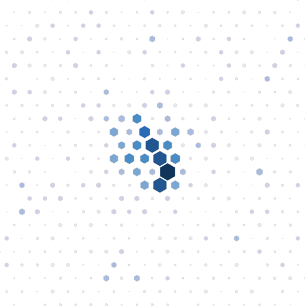
In addition to size and saturation/value, alpha (opacity) could also be used to represent a hex attribute (see the bottom of this example page for a value-by-alpha representation of density above a Google map).
Implementation
As noted above, hexbins have been implemented in a few statistical packages, including R. But I haven’t seen any other implementations, and certainly not a client-side one. At first I tried to just port the R code, but it made no sense to me, and included many dependencies within R. So I decided I’d have to roll my own. Rolling my own seemed really hard, so luckily I ran into Alex Tingle’s libhex library. Though certainly not designed for hex-binning (I believe it was made with game developers in mind), this great library has all the methods necessary to create a hexagonal lattice data structure. And though written in C++, the author had completed an experimental JavaScript version.
It took some back-and-forth with libhex’s author Alex to figure it out, but the library’s methods make it easy to create a hexagonal lattice or grid of a given size with specified hexagon size. Once created, the Grid.Hex method can be used to determine corresponding hexes for each 2D point in the dataset to be binned. After this is achieved, we have a hexagonal lattice data structure, with each hex in the grid storing the points contained within its data space.
This creates the data structure, and performs the necessary binning routine for each point, but the library wasn’t meant to render anything. I therefore paired it with my favorite data-driven visualization (or document-manipulation) library, D3.js. The result is d3.hexbin.js, which can be used like so:
.xValue( function(d) { return d.x; } )
.yValue( function(d) { return d.y; } )
.hexI( hexI )
( data );
The result returned by d3.layout.hexbin() — hexset in the above — is simply an array of hex objects with important properties — notably data (the binned points for the particular hex) and pointString (a string representing the outline points of the hex). As far as symbolization, once the hexbinning routine is completed, representing the data with multiple symbologies is quite easy with D3. The example posted here shows off the exact same random data represented with dots, choropleth, proportional symbol, bivariate, and value-by-alpha symbologies. The code below is used to render the frequency hexgrid as a choropleth.
.append( "svg:svg" )
.append( "svg:g" )
.attr( "class", cbScheme + " stroke-true" )
.selectAll( "polygon" )
.data( hexset )
.enter().append( "svg:polygon" )
.attr( "class", function(d)
{
return 'q'
+ ( (numClasses-1) - scale(d.data.length))
+ "-" + numClasses;
})
.attr( "points", function(d)
{
return d.pointString;
});
All the code is stored in the hexbin-js Github repository. Please browse the src and tests folders to see more of what’s going on here.
Because I’m a cartographer (or something), I wanted to create a geographic proof-of-concept for this method. I came up with this, combining my custom hexbin layout class with D3.js and Polymaps. The resultant interactive visualization shows an overview + focus view of all Walmarts in the USA. Hexes can be moused over for a focus view.
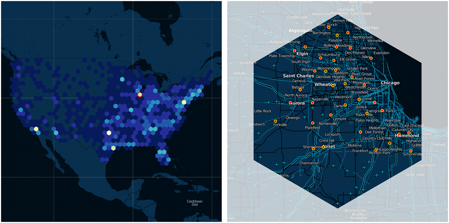
d3.layout.hexbin requires D3.js, though the dependencies don’t go that deep, so a few quick mods would allow you to use the hexbinning methods with any JavaScript mapping or graphics library. Use as you will. Many thanks to both Alex Tingle and Mike Bostock for answering my questions.
16 Comments
Very Cool!
Cool post - love working with hexagons. There is some cool work on the quant side done by Kevin Sahr using a Icosahedral Snyder Equal Area (ISEA) projection. More here http://webpages.sou.edu/~sahrk/dgg/. We uploaded a bunch of hexagons at different zoom levels on GeoCommons:
http://geocommons.com/search?limit=10&mh_query=hexagons&model=Overlay&page=1&query=hexagons
Nice post, just a few comments. The primary advantage of binning is speed. Smoothing methods have come a long way, and can handle large data sets using tensor products. If data sets are still too large, binning combined with smoothing, using bin counts as the response can produce feature rich plots. I was not aware of Adler’s book, but in his example he uses a bin size that is too small and fails to accentuate the clustering of points along the lower right of the data cloud. High concentrations would show up better as a smooth bivariate density. Where hexagons are useful is for sampling, Dennis White has written about hexagonal grids in mapping applications.
Thanks for providing this. Fantastic.
Just as a small addition - in order for the examples to work in firefox, you need to add width and height to the svg element.
.append( “svg:svg” ).attr(’width’, ‘100%’).attr(’height’, ‘100%’)
Thanks again… great stuff.
Hi there, I wish for to subscribe for this web site to get latest updates, thus where can i do it please
assist.
Great stuff.
FYI, your link to the example of value-by-alpha representation of density above a Google map links to a file on your computer, presumably, which does me no good.
I do believe all of the ideas you’ve presented for your post. They are very convincing and will certainly work. Nonetheless, the posts are very short for newbies. Could you please prolong them a little from next time? Thank you for the post.
Hi Zachary, Great imputs from your breif explanation on the techniques of using interlocking hexagons to aggregate 2-dimensional data- the Hexagonal binning.
Got to learn lots.
Hey Zachary., I use indiemaps for navigation, and am in absolute appreciation of it.
I visited various sites however the audio quality for audio songs existing at this web
page is genuinely excellent.
Wow! After all I got a website from where I be able to in
fact obtain helpful information regarding my study and knowledge.
Very rapidly this website will be famous amid all blogging viewers, due to it’s fastidious articles or
reviews
Water often is used as a base for your favourite low carb smoothie; it owns the minimum amount of carbs of most -infact zero.
These “smoothies” are used in lieu of meals during the day.
They keep the immune system healthy and strong as they ward off infections and heal cuts and
wounds.
Fantastic goods from you, man. I have understand your stuff previous to and you are just too wonderful.
I really like what you have acquired here, certainly like what you are stating and the way in which you say it.
You make it enjoyable and you still care for to keep it wise.
I cant wait to read much more from you. This is actually a wonderful website.
I merely weren’t able to get away from your web blog ahead of indicating i basically appreciated the typical data anyone source for your attendees? Shall be once more continuously in order to look at fresh threads
8 Trackbacks
[...] about HexBin and much more detailed information about its geographical implementation can be found here. Tags: design, [...]
[...] story about HexBin and most some-more minute information about the geographical doing can be found here. Tags: clutter, com, d3, Data, design, forest johnson, function, Grid, hexagonal grid, HexBin, [...]
[...] All about hexagonal binning (hexbins) Hexagonal binning demo on GitHub by the author Uses the D3 javascript library, and as such, it is incompatible with IE6/7/8 [...]
[...]
[...] What are Hexbins? And what is binning? [...]
[...] First of all we’re going to be using D3.js along with hexbins.js. You can read a lot about hexbins.js here. [...]
[...] scatterplot, within the last few years hexbinning has been used more and more in cartography. (See this great blog post by Zachary Forest Johnson which traces this history and explains how to do create hexbin maps using [...]
[...] an online tool that is capable of producing non conventional charts such as Dendrograms, Treemaps, Hexagonal Binnings and Alluvial [...]
[...] Hexbins! [...]