I’m happy to be doing less Flash and more JavaScript development these days. In particular, I’ve been investigating two open-source JavaScript web mapping platforms: one old, OpenLayers, and one new, Polymaps.
OpenLayers has been around a while, but still performs remarkably well as a slippy map framework while allowing easy thematic map customization. Polymaps is brand new (from Stamen so you know it’s going to blow your mind), but is remarkable for enabling web standards-based thematic customization of geographic layers loaded via GeoJSON or KML onto “vector tiles that are rendered with SVG”.
In this post I show how either OpenLayers or Polymaps can be used to create dynamic and customizable noncontiguous cartograms with very little code.
Idea
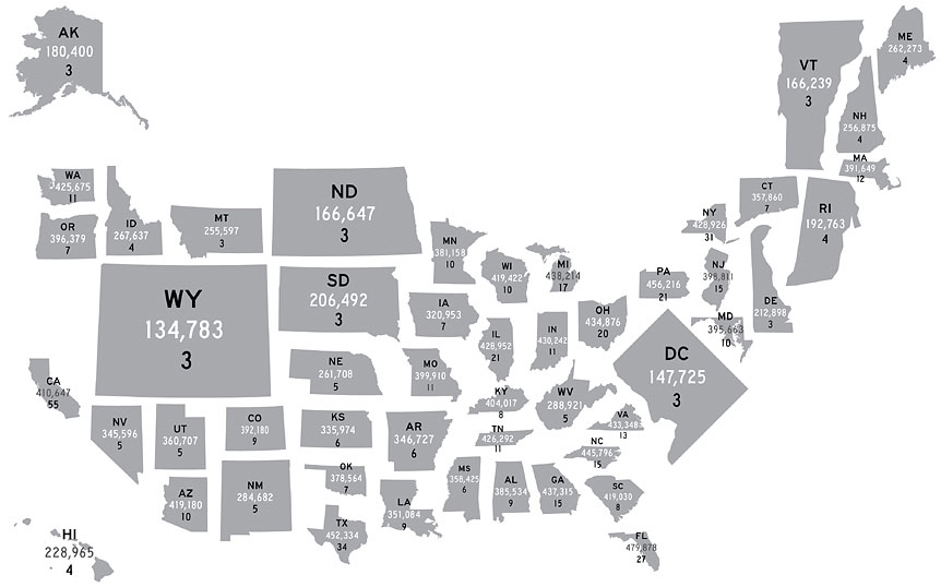
The above is a cartogram of state electoral influence from 2007 by the NY Times
I’ve written about these gals before. The form involves resizing features (like states or countries) relative to the units’ attribute values in a given field (often population). Unlike the more common, contiguous form of the cartogram, noncontiguous cartograms don’t attempt to maintain topology, but are therefore free to maintain shape perfectly and experiment with position, as in the above example.
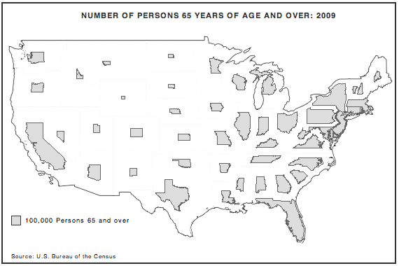
Here’s an example from Judy Olson’s original 1976 article on this cartogram form.
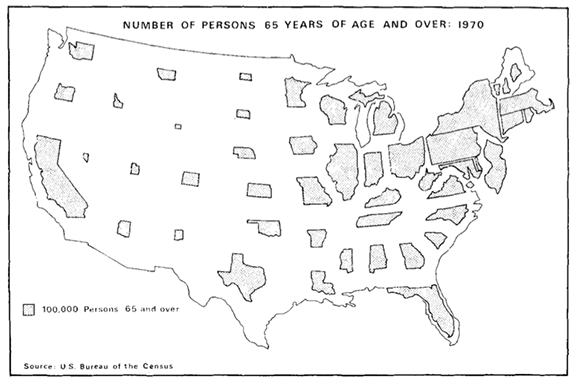
See my older post or Olson’s article for more info on the technique and the theory behind it. Olson produced the above image semi-manually using a projector — each state was projected at a precise scaling factor and then traced. Below I show how to do more or less the same thing, but with JavaScript and either OpenLayers or Polymaps.
Implementation
I wanted to be able to load in any polygonal geodata file (supported by the chosen web mapping framework) and resize the features based on any numerical attribute in order to form a noncontiguous cartogram. The advantage of implementing this within a web mapping framework is obviously that additional data layers from various sources can easily be over or underlain.
As a test and proof of concept for both frameworks, I wanted to reproduce Olson’s graphic (above) as best as I fairly easily could. Olson used 1970 Census data to show the number of people aged 65+ by state; here I’m updating it with estimated 2009 data. Specifically, I’ll be loading this Geocommons data layer uploaded last year.
I’ve been working with OpenLayers for about half a year so I implemented cartograms there first.
OpenLayers
Implementing noncontiguous cartograms in OpenLayers is fairly straightforward, thanks to the helpful methods provided by this comprehensive framework. The first step is loading the geodata.
Load geodata
OpenLayers makes loading geodata quite easy; the library can parse WKT, GML, KML, GeoJSON, GeoRSS, etc. For all we’re gonna use the Layer.Vector class. In this case I’ll load in the KML version from Geocommons, and therefore OpenLayer’s Format.KML parser.
projection : new OpenLayers.Projection("EPSG:4326"),
strategies: [ new OpenLayers.Strategy.Fixed() ],
protocol: new OpenLayers.Protocol.HTTP( {
url: "http://geocommons.com/overlays/55629.kml",
format: new OpenLayers.Format.KML( {
extractStyles: false,
extractAttributes: true,
maxDepth: 2
} )
} ),
style : {
'fillColor' : '#dddddd', 'fillOpacity' : 1,
'strokeColor' : '#666666', 'strokeWidth' : 1
}
} );
Noncontiguous cartograms don’t require a geographic projection — regardless of the projection of the original linework the features can still be scaled up or down accurately to form the cartogram. So the only reasons for projection are aesthetics and to enhance recognizability of features. I’m unsure of what projection Olson used, but I just went for that old classic, Albers Equal Area. Specifically, I used Proj4js and the following definition:
Proj4js.defs["MY_ALBERS"] = “+proj=aea +lat_1=32 +lat_2=58 +lat_0=45 +lon_0=-97 +x_0=0 +y_0=0 +ellps=WGS84 +datum=WGS84 +units=m +no_defs”;
To apply it, I just create a new OpenLayers.Projection which gets applied to the map when it’s instantiated. Thematicmapping.org has more info on projections and OpenLayers.
Unless you already know the maximum value of whatever attribute you’re mapping, you’ll have to loop through them all once before you can loop through them again to scale. Attributes are accessible via the attributes property of each OpenLayers.Feature.Vector (accessible via the features property of the OpenLayers.Layer.Vector).
Scale features
In order to scale a polygonal feature for a noncontiguous cartogram, we must know:
- the feature’s value for the chosen thematic attribute (see above)
- the feature’s area and centroid as rendered
OpenLayers makes these easily accessible. Each feature’s geometry object has getArea and getCentroid methods. As far as I can tell, the getCentroid function returns the true polygonal center of mass, and not just the center of the feature’s bounding box.
- the feature’s desired area (in pixels) given the maximum area provided and the feature’s value as a percentage of the layer’s maximum value
desiredArea = ( value / maxValue ) * maxArea;
- finally, the feature’s scale which is just a function of its original and desired area
desiredScale = Math.sqrt( desiredArea / originalArea );
This scale is then applied via the resize method of each feature’s geometry.
feature.geometry.resize( desiredScale, centroid );
Result
Here’s an image from the example you can find on this page. All source can just be accessed from there.
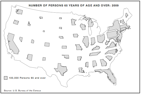
Hey, that looks pretty great. Michigan’s kinda off-center, but I believe that’s because the polygon is only defined by one ring of coordinates, though it should be a multipolygon. Perhaps more noticeable is the overlap in the Northeast. In Judy Olson’s original example, states were blown up by a visual projector and then traced. But the projector could be aimed before tracing, thus avoiding overlap. In this case I simply scale the states and keep them at their original centroids.
I could avoid overlap by determining appropriate positioning and setting this within OpenLayers (but overlap would be very difficult to determine and then address dynamically) or by significantly reducing the configurable maximum area allowable on the resultant cartogram (but in order to be sure you’re preventing overlap features would have to be scaled quite small, which would detract from the readability of the cartogram).
Polymaps
Polymaps is a fairly new JavaScript mapping library by Stamen and SimpleGeo. Geocommons recently introduced Polymaps to their online mapping service, creating a quite powerful Flash-free online thematic mapping tool. Creating noncontiguous cartograms in Polymaps was a bit tougher than the process detailed above, just because the library is so light-weight.
Load geodata
The first step is quite easy. As far as vector geodata formats, Polymaps only has built-in support for GeoJSON, though they do provide a KML example that takes advantage of an optional fetch method specified in the GeoJSON layer constructor.
But I’ll just go with GeoJSON for this one. I found out in this post from GeoIQ that I can access a GeoJSON version of features in any Geocommons dataset by going to the “features.json” endpoint. So for my 2009 estimated census dataset I’ll be loading in http://geocommons.com/overlays/55629/features.json?geojson=1 using the following simple method:
map.add(po.geoJson()
.url(url)
.on("load", load)
.tile( false )
.id("states"));
Note that loading directly from Geocommons only works while developing locally because of cross-domain policy. So in my finished example I end up loading a local version of the JSON.
Polymaps is limited to the Web Mercator projection for display, but we can still produce a passable reproduction of Olson’s original.
As in the OpenLayers example above, unless you already know the maximum value of your attribute, you’ll need to first loop through the features to determine it. In the above code, you can see I’m using the layer’s on method to listen for the “load” event. And in there I can get my features off the event object’s features property. Attributes are stored on each feature’s data.properties property.
Scale features
To scale each feature we must first know it’s value in the chosen attribute (see above). Then we need to determine it’s current area (in pixels) in order to figure the feature’s desired area on the eventual cartogram. OpenLayers provides a convenient method for this but in Polymaps we have to roll our own; for this Mike Bostock (one of the primary authors of Polymaps) was of much help. To calculate the area of each feature I just needed access to the list of projected coordinates (then I could employ the basic technique detailed here). Mr. Bostock pointed me to the pathSegList property of the SVGPathElement interface. The pathSegList exposes a list of path segments with the SVGPathSeg interface. Mike said I could count on these segments being one of types “M” (move to), “L” (line to), or “Z” (end line). With this information I quickly put together a method that should return the projected area of any SVGPathElement that Polymaps may produce.
{
var area = 0;
var seg1, seg2;
var nPts = segList.numberOfItems;
// let's see if the last item is a 'Z' (it should be)
var lastLetter =
segList.getItem( nPts - 1 ).pathSegTypeAsLetter;
if ( lastLetter.toLowerCase() == 'z' )
nPts --;
var j = nPts - 1;
segItem_list:
for ( var i = 0; i < nPts; j=i++ )
{
seg1 = segList.getItem( i );
seg2 = segList.getItem( j );
area += seg1.x * seg2.y;
area -= seg1.y * seg2.x;
}
area /= 2;
return Math.abs( area );
}
I could easily create a similar centroid method, but I got lazy and decided to just use the center of each feature’s bounding box (accessible via each feature SVG element’s getBBox method).
The desired area and scale are calculated just as we did above in OpenLayers:
desiredArea = ( value / maxValue ) * maxArea;
desiredScale = Math.sqrt( desiredArea / originalArea );
The scale is then applied via the ‘transform’ attribute of each SVG element; both scale and x-y translation must be defined in the ‘transform’ attribute:
"transform",
"scale(" + scale + " " + scale + ")" + " " +
"translate(" +
-( ( centerX * scale - centerX ) / scale ) +
" " +
-( ( centerY * scale - centerY ) / scale ) +
")"
);
Result
As before, here’s an image captured from the example you can find on this page. You’ll see a bit of the code there, but please ‘view source’ to see all the code and markup.
Aside from the necessary difference of projection, the main thing that stands out is the overlap in the Northeast. I discussed possible ways to avoid this in the OpenLayers example above.
Conclusion
Nothing here is new. I’ve been doing this in Flash for a while — see here and here; and of course Judy Olson was doing it some 35 years ago. But it’s nice to see it working dynamically in a couple of open source, web standards-compliant libraries. Thanks to OpenLayers, Polymaps, and Geocommmons for making it possible!